

Processing Sound Files for Emotion Recognition
This article will explore the key steps involved in processing sound files for emotion recognition, including reading audio data, extracting relevant
Sound files contain a wealth of information that can be used to recognize emotions in speech. By analyzing various acoustic features of speech recordings, we can extract meaningful data to train machine learning models for emotion classification. This article will explore the key steps involved in processing sound files for emotion recognition, including reading audio data, extracting relevant features, dealing with challenges like noise and multiple speakers, and preparing the data for machine learning.
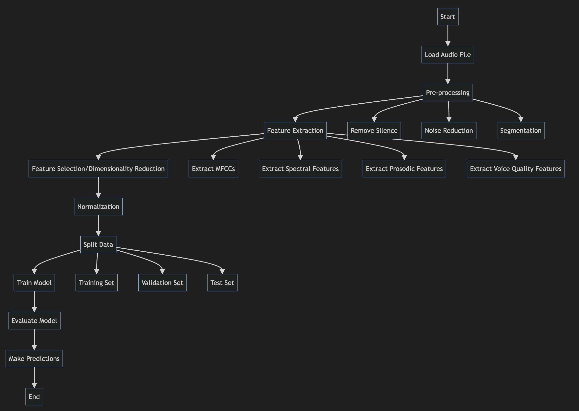
Sound File Formats and Data
Sound files typically store audio data as a series of samples representing the amplitude of the sound wave at fixed time intervals. Common formats include:
WAV: Uncompressed audio, high quality but large file sizes
MP3: Compressed audio, smaller files but some loss of quality
FLAC: Lossless compressed audio, preserves quality with smaller files
AAC: Compressed audio, alternative to MP3
The key data contained in sound files includes:
Sample rate: Number of samples per second (e.g. 44.1 kHz)
Bit depth: Number of bits per sample (e.g. 16-bit)
Number of channels: Mono (1) or stereo (2)
Audio samples: Series of integers representing wave amplitude
Python Libraries for Audio Processing
Several Python libraries are useful for working with audio files:
librosa: Feature extraction, loading audio files
pydub: Audio file manipulation
scipy: Signal processing functions
pyAudioAnalysis: Audio feature extraction and classification
soundfile: Reading/writing sound files
wavio: Reading/writing WAV files
librosa is particularly well-suited for audio analysis tasks. Here's an example of loading a WAV file with librosa:
import librosa

# Load audio file
y, sr = librosa.load('speech.wav')

# y = audio time series
# sr = sampling rate
Feature Extraction
To recognize emotions, we need to extract relevant acoustic features from the raw audio data. Some key features include:
Mel-frequency cepstral coefficients (MFCCs): Represent the short-term power spectrum
Spectral features: Spectral centroid, spectral flux, spectral rolloff
Prosodic features:
Pitch (fundamental frequency)
Energy/intensity
Speaking rate
Voice quality features:
Jitter
Shimmer
Harmonics-to-noise ratio
Here's an example of extracting MFCCs using librosa:
import librosa

y, sr = librosa.load('speech.wav')

# Extract 13 MFCCs
mfccs = librosa.feature.mfcc(y=y, sr=sr, n_mfcc=13)
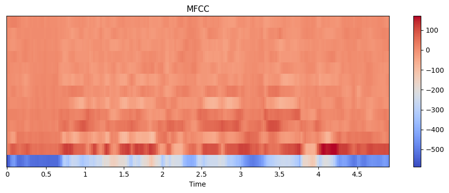
We can visualize the MFCCs:
import librosa
import librosa.display
import matplotlib.pyplot as plt

y, sr = librosa.load('speech.wav')
mfccs = librosa.feature.mfcc(y=y, sr=sr, n_mfcc=13)

plt.figure(figsize=(10, 4))
librosa.display.specshow(mfccs, x_axis='time')
plt.colorbar()
plt.title('MFCC')
plt.tight_layout()
plt.show()
This produces a visualization like:
Extracting multiple features:
import numpy as np
import librosa

def extract_features(file_path):
    y, sr = librosa.load(file_path)

    # MFCCs
    mfccs = np.mean(librosa.feature.mfcc(y=y, sr=sr, n_mfcc=13).T, axis=0)

    # Spectral features
    spectral_centroid = np.mean(librosa.feature.spectral_centroid(y=y, sr=sr).T, axis=0)
    spectral_rolloff = np.mean(librosa.feature.spectral_rolloff(y=y, sr=sr).T, axis=0)

    # Prosodic features
    pitch = np.mean(librosa.yin(y, fmin=librosa.note_to_hz('C2'), fmax=librosa.note_to_hz('C7')))
    energy = np.mean(librosa.feature.rms(y=y))

    return np.concatenate((mfccs, spectral_centroid, spectral_rolloff, [pitch], [energy]))

features = extract_features('speech.wav')
Challenges in Audio Processing
Several challenges arise when working with speech audio for emotion recognition:
- Background Noise
Background noise can significantly impact the extracted features. Some strategies to handle noise include:
Noise reduction algorithms
Voice activity detection to isolate speech segments
Spectral subtraction
Wiener filtering
Example of noise reduction with noisereduce library:
import noisereduce as nr
import soundfile as sf

# Load audio
y, sr = sf.read("noisy_speech.wav")

# Perform noise reduction
reduced_noise = nr.reduce_noise(y=y, sr=sr)

# Save denoised audio
sf.write("denoised_speech.wav", reduced_noise, sr)
- Multiple Speakers
Dialogues or group conversations present the challenge of separating individual speakers. Techniques to address this include:
Speaker diarization: Segmenting audio by speaker
Source separation algorithms
Beamforming (for multi-microphone recordings)
Example using pyannote for speaker diarization:
from pyannote.audio import Pipeline

pipeline = Pipeline.from_pretrained("pyannote/speaker-diarization")

# Apply diarization
diarization = pipeline("conversation.wav")

# Print results
for turn, _, speaker in diarization.itertracks(yield_label=True):
    print(f"start={turn.start:.1f}s stop={turn.end:.1f}s speaker_{speaker}")
- Emotion Ambiguity
Emotions are subjective and can be ambiguous or mixed. Strategies include:
Using dimensional emotion models (valence-arousal)
Multi-label classification
Fuzzy classification approaches
- Individual Variability
Speaking styles and emotional expressions vary between individuals. Approaches to handle this:
Speaker normalization techniques
Transfer learning
Large diverse datasets
- Context Dependence
Emotions depend on linguistic and situational context. Potential solutions:
Multimodal approaches (combining speech with text/video)
Including contextual features
Sequence modeling (e.g. using RNNs/LSTMs)
Data Preparation for Machine Learning
After feature extraction, several steps prepare the data for training emotion recognition models:
- Segmentation: Divide audio into fixed-length segments or utterances
import librosa

def segment_audio(file_path, segment_length=3.0):
    y, sr = librosa.load(file_path)

    segments = []
    for start in range(0, len(y), int(segment_length * sr)):
        end = start + int(segment_length * sr)
        if end <= len(y):
            segment = y[start:end]
            segments.append(segment)

    return segments

segments = segment_audio('long_speech.wav')
- Normalization: Scale features to a common range
from sklearn.preprocessing import StandardScaler

scaler = StandardScaler()
normalized_features = scaler.fit_transform(features)
- Dimensionality Reduction: Reduce feature set size (optional)
from sklearn.decomposition import PCA

pca = PCA(n_components=10)
reduced_features = pca.fit_transform(normalized_features)
- Train-Test Split: Divide data into training and testing sets
from sklearn.model_selection import train_test_split

X_train, X_test, y_train, y_test = train_test_split(features, labels, test_size=0.2, random_state=42)
- Data Augmentation: Generate additional training samples (optional)
import nlpaug.augmenter.audio as naa

aug = naa.PitchAug(factor=(0.8, 1.2))
augmented_audio = aug.augment(y)
Machine Learning for Emotion Recognition
With the prepared data, we can train machine learning models for emotion classification. Common approaches include:
- Traditional ML: SVM, Random Forests, Gradient Boosting
from sklearn.ensemble import RandomForestClassifier

rf_model = RandomForestClassifier(n_estimators=100)
rf_model.fit(X_train, y_train)

predictions = rf_model.predict(X_test)
- Deep Learning: CNNs, RNNs, Transformer models
import tensorflow as tf

model = tf.keras.Sequential([
    tf.keras.layers.Dense(64, activation='relu', input_shape=(num_features,)),
    tf.keras.layers.Dense(32, activation='relu'),
    tf.keras.layers.Dense(num_emotions, activation='softmax')
])

model.compile(optimizer='adam', loss='categorical_crossentropy', metrics=['accuracy'])
model.fit(X_train, y_train, epochs=50, batch_size=32, validation_split=0.2)
- Transfer Learning: Use pre-trained audio models
import tensorflow_hub as hub

yamnet_model = hub.load('https://tfhub.dev/google/yamnet/1')

def extract_embeddings(file_path):
    y, sr = librosa.load(file_path, sr=16000)
    scores, embeddings, spectrogram = yamnet_model(y)
    return np.mean(embeddings, axis=0)

embeddings = extract_embeddings('speech.wav')
Conclusion
Processing sound files for emotion recognition involves multiple steps, from loading audio data to extracting relevant features and preparing the data for machine learning. While challenges like noise and speaker variability exist, various techniques and tools are available to address these issues. By leveraging libraries like librosa and applying appropriate pre-processing and feature extraction methods, researchers can effectively analyze speech audio for emotional content. As the field advances, multimodal approaches and more sophisticated deep learning models are likely to further improve emotion recognition accuracy.


